Author Archive

We took a retired Siemens A36 cellphone to learn the capabilities of this new Siglent scope. Available documentation and medium-density PCB of the selected A36 made the signal probing easy to implement. We used TEK P6243 active probes initially for their low capacity loading but changed to passive probes later as monitored signals proved to be quite robust.


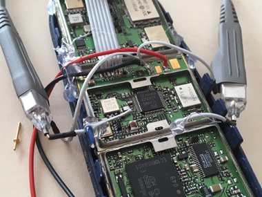
Figure 1: probing IQ signals in Tx and Rx path of the Siemens A36


Three signals were selected to monitor the cellphone operation:

  1. Transmit IQ baseband modulation signal, Q component, on Pin 48 on scope Channel 1
  2. Receive IQ baseband modulation signal, I component, on Pin 12 on scope Channel 2
  3. Battery current consumption from 0.1 Ohm resistor, between (-) power supply and phone ground on scope Channel 4 (resulting in negative signal polarity)


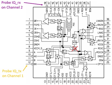
Figure 2: block diagram of PMB6250 Smarti IC with probe inputs

At first we observed the phone attached to the GSM network, periodically listening for an eventual incoming call on paging channel once per second. Once every 33 seconds, the phone is additionally checking the signal level of other base stations to request the network to camp on the stronger base station in the case when the phone is moving.


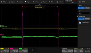
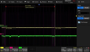
Figure 3: Rx signals for paging (left) and neighbour cell measurements (right)

Current peaks of 30 mA at the end of Rx signal burst indicate the processing power needed for decoding of the received signal. Neighbour channel measurement need only a part of the burst, allowing for frequency switching (PLL re-tuning) between the 3 bursts. We can see how noisy the other base stations are, and that the first burst of the serving base station has the least noise of all.


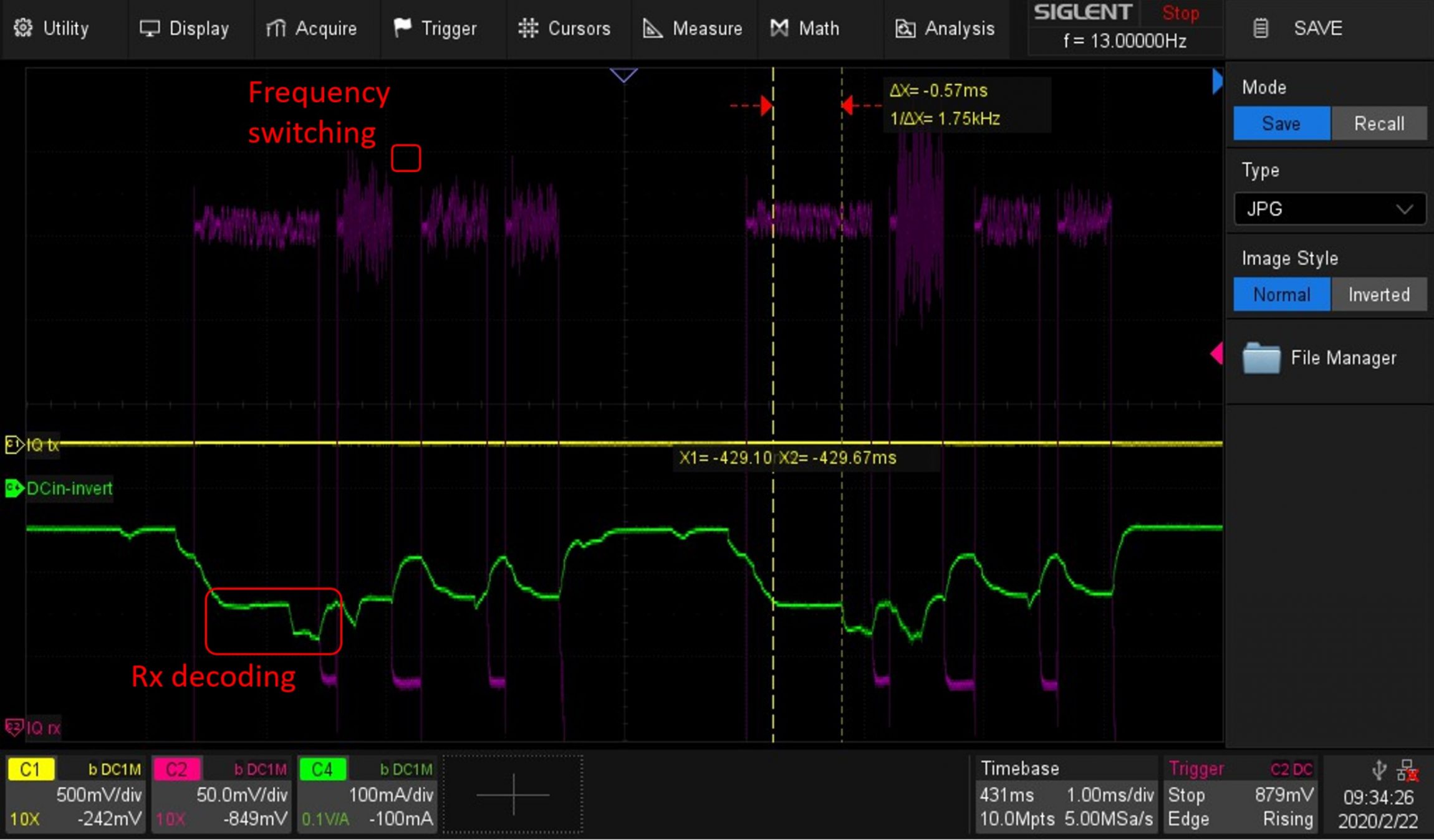
Figure 4: Rx signal detail and processing power (power consumption)

Using the scope persistence and colour histogram, we can visualise the received signal. We also used the scope Zone Trigger function (area 1) to distinguish between the longer data and shorter paging channels. We see the signal reception is longer than the data burst length of 570 µs. This allows for the demodulation of signals that may be dealing with multipath propagation. In a mountainous region, for example, base station signals can reach the phone on the direct fast track but may also propagate along a path with multiple reflections. Up to +-3 symbols delay can be processed by the A36 channel equaliser.


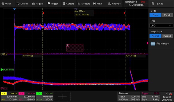
Figure 5: Histogram of Rx signal with 1 sec persistence

Then we set up a call between the phone and the network. For the first time, we can see the phone transmitter operation (yellow Channel 1). As the phone receives an incoming call from the paging channel it changes from idle to the call state after the user picks up the call of the ringing phone.


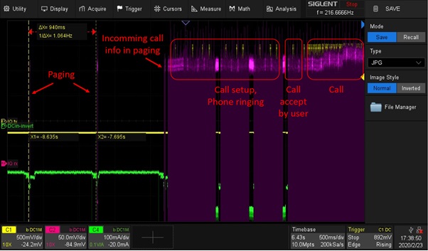
Figure 6: Incoming call setup flow

Parallel to the call, the phone still performs neighbour cell measurements for the case it finds a stronger base station that can handover the call.


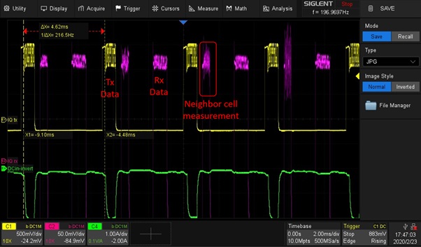
Figure 7: Call Tx and Rx bursts

On the transmit burst we can observe the permanently changing data bits carrying the speech signal. The static non-changing bits are the Tail Bits at the beginning and the end of the burst. Most important is the Training Sequence in the middle of the burst. The channel equaliser of the receiver is training its best adjustments on this training sequence and use this adjustment for the whole burst. The training sequence is in the middle of the burst, while the propagation conditions are changing as the phone is moving and the position in the middle of the burst is best for the whole burst. 1-second persistence, colour histogram and zone trigger features of the scope are used to visualise this dynamic situation.


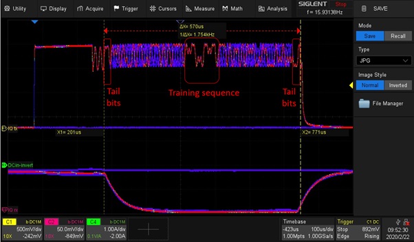
Figure 8: Histogram of Tx signal with 1-sec persistence

Peak current of almost 2 A at 4 V DCin covers the demand of the Tx power amplifier. During the reception of a call, the peak current is 100 mA. There is no measurable power consumption between the Rx paging reception, the implemented Eco-Mode only powers the 32 kHz clock inside the phone to wake-up the phone for the next paging. That’s why the battery charge can last for many days if no calls performed.

Large memory depth of the scope was very helpful to zoom-in into the captured data. Various trigger options helped to get a stable trigger for fast-changing signals.

We were extremely surprised by the good performance and rich features of the new Siglent SDS2000x Plus oscilloscope. The performance of this mid-class entry model is on the level of high-end units back in the time when one of the authors designed the A36 phone. We recommend this scope to all interested readers and look forward to checking LTE and 5G phones with this scope in our next projects.

Products Mentioned In This Article:

Analysing GSM Radio Protocol with a Siglent SDS2000X Plus Oscilloscope

Posted on: August 20th, 2021 by James
Analysing GSM Radio Protocol with a Siglent SDS2000X Plus Oscilloscope 20th August 2021
We took a retired Siemens A36 cellphone to learn the capabilities of this new Siglent scope. Available documentation and medium-density PCB of the selected A36 made the signal probing easy to implement. We used TEK P6243 active probes initially for their low capacity loading but changed to passive probes later as monitored signals proved to be quite robust.   ...

Programming Example: Retrieve data from an XE series Oscilloscope using Kotlin

Posted on: August 20th, 2021 by James
Programming Example: Retrieve data from an XE series Oscilloscope using Kotlin 20th August 2021
The SDS series of oscilloscopes all feature remote programming and data collection capabilities. They can be integrated easily into many automated test environments to ease the setup and data acquisition during testing. One of our helpful customers developed a nice programming example designed to set up and retrieve data from a SIGLENT SDS1202X-E Oscilloscope using Kotlin, a free open source c...

Comparison / Differences between the SDS1000X and SDS1000X-E oscilloscope families

Posted on: August 20th, 2021 by James
Comparison / Differences between the SDS1000X and SDS1000X-E oscilloscope families 20th August 2021
The short list of differences between the X and the 2 channel XE (SDSs1202XE) is as follows: – X has 50 ohm/ 1 MOhm selectable input impedance. XE only has 1 MOhm fixed. You will need a 50 ohm matching through adapter if you wish to connect to 50 Ohm circuits/minimize reflections. – The X has a slightly larger display (8″)  vs. the XE (7″) ...

Programming Example: List connected VISA compatible resources using PyVISA

Posted on: August 20th, 2021 by James
Programming Example: List connected VISA compatible resources using PyVISA 20th August 2021
PyVISA is a software library that enables Python applications to communicate with resources (typically instruments) connected to a controlling computer using different buses, including: GPIB, RS-232, LAN, and USB. This example scans and lists the available resources. It requires PyVISA to be installed (see the PyVISA documentation for more information) *** #Example that scans a compute...

SDS FFT performance on low frequency signals

Posted on: August 20th, 2021 by James
SDS FFT performance on low frequency signals 20th August 2021
Like many modern oscilloscopes, the SIGLENT SDS series feature FFT math functions that calculate frequency information from the acquired voltage vs. time data. FFT stands for Fast Fourier Transform, and is a common method for determining the frequency content of a time-varying signal. Converting time domain data to the frequency domain makes measuring characteristics like phase noise and harmonics...

Programming Example: SDS Oscilloscope screen image capture using Python over LAN

Posted on: August 20th, 2021 by James
Programming Example: SDS Oscilloscope screen image capture using Python over LAN 20th August 2021
Here is a brief code example written in Python 3.4 that uses a socket to pull a display image (screenshot) from a SIGLENT SDS1000X-E scope via LAN and save it to the local drive of the controlling computer. NOTE: This program saves the picture/display image file in the same directory that the .py file is being run from. It will overwrite any existing file that has the same na...

Measuring Power Supply Control Loop Response with Bode Plot II

Posted on: August 20th, 2021 by James
Measuring Power Supply Control Loop Response with Bode Plot II 20th August 2021
Introduction Stability is one of the most important characteristics in power supply design. Traditionally, stability measurements require expensive frequency response analysers (FRA) which are not always available in a laboratory. SIGLENT has released Bode Plot â…ˇ features to the SIGLENT SDS1104X-E, SDS1204X-E, SDS2000X-E, SDS2000X Plus, an...

Measuring the Modulation Index of an AM Signal using an FFT

Posted on: August 20th, 2021 by James
Measuring the Modulation Index of an AM Signal using an FFT 20th August 2021
Introduction In AM schemes, the modulation index refers to the amplitude ratio of the modulating signal to the carrier signal. With the help of Fast-Fourier-Transforms (FFT), the modulation index can be obtained by measuring the sideband amplitude and the carrier amplitude. In this application note, we are going to show a convenient method of ...

Programming Example: SDS Oscilloscope save a copy of a screen image via Python/PyVISA

Posted on: August 20th, 2021 by James
Programming Example: SDS Oscilloscope save a copy of a screen image via Python/PyVISA 20th August 2021
Here is a brief code example written in Python 3.4 that uses PyVISA to pull a display image (screenshot) from a SIGLENT SDS oscilloscope via USB and save it to a drive on the controlling computer. NOTE: This program saves the picture/display image file to the E: drive, which may or may not exist on the specific computer being used to run the application. Download Python 3.4...

Power Supply Design: Load Step Response with a SIGLENT DC Electronic Load

Posted on: August 20th, 2021 by James
Power Supply Design: Load Step Response with a SIGLENT DC Electronic Load 20th August 2021
Building a power supply that can handle various loads without oscillating can be a challenge. Computational models and computer simulations can help get your design headed in the right direction, but physical testing is essential to proving the performance of your design. One method of quickly determining stability is to use a load step response. In this test, a DC electronic load is used to...

Sub Categories

Blog (40)

Siglent Oscilloscope Offers (1)

CLICK TO CALL

0118 9786911
CLICK TO EMAIL